PSD Visualization

The PSD data computed with psysmon can be used to compute spectrograms of various length, from hours, to days or weeks. These plots are useful to assess the data quality and gives an overview of the signals of the data set.

The PSD data computed in the chapter Power Spectral Density is used to create a spectrograms for various time spans. We will create a daily and weekly spectrograms, as well as one for the whole time range of available data.

Create the output directory

We will save the spectrogram images in a dedicated output directory. Create the directory psd_images in the psysmon_output folder of the tutorial directory structure.

stefan@hausmeister:~/tutorial/psysmon_output$ mkdir psd_images
stefan@hausmeister:~/tutorial/psysmon_output$ tree -L 1
.
├── availability
├── psd_data
└── psd_images

3 directories, 0 files
stefan@hausmeister:~/tutorial/psysmon_output$ 

Create the psd visualization collection

Create a collection named psd visualization and add the collection node create psd images to the collection.

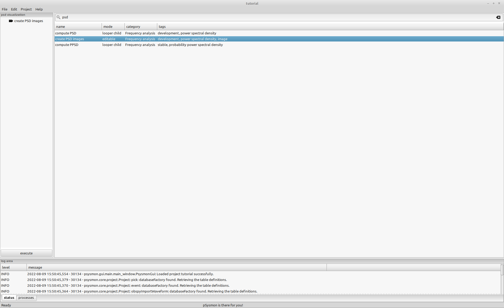
Edit the create psd images preferences

Open the create psd images preferences dialog using the context menu in the collection listbox. Enter the following parameters in the three available pages and confirm them by clicking the OK button.

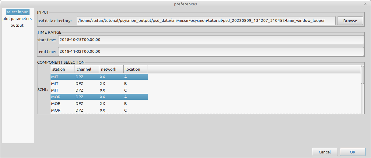
select input

psd data directory

Select the output directory of the psd computation collection. The directory containing the psd directory has to be selected. In my case this directory is located in /home/stefan/tutorial/psysmon_output/psd_data/smi-mr.sm-psysmon-tutorial-psd_20220809_134207_310452-time_window_looper.

start time

The start time of the visualization (2018-10-25T00:00:00).

end time

The end time of the visualization (2018-11-02T00:00:00).

SCNL

The components that should be visualized (MIT:DPZ:XX:A, MOR:DPZ:XX:A)

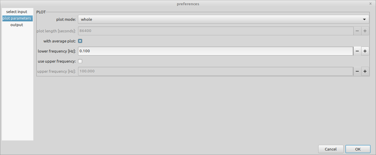
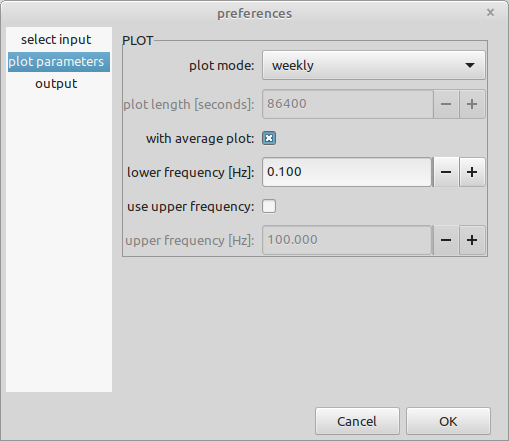
plot parameters

plot mode

The fragmentation of the selected time span. An image is created for each fragment (whole).

with average plot

Add an average plot to the spectrograms (checked).

lower frequency [Hz]

The lower frequency limit of the spectrogram (0.1)

use upper frequency

Use an upper frequency limit for the spectrogram (unchecked)

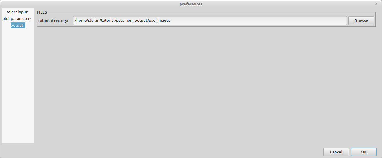
output

output directory

The output directory where the created spectrogram images will be saved (the psd_images directory created above).

Execute the collection

Execute the collection by clicking the execute button and check the process execution in the processes tab of the log area.

Inspect the output

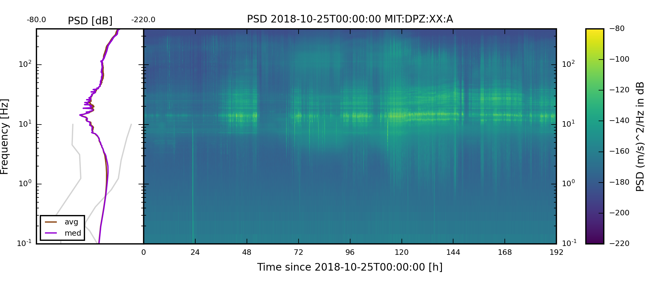
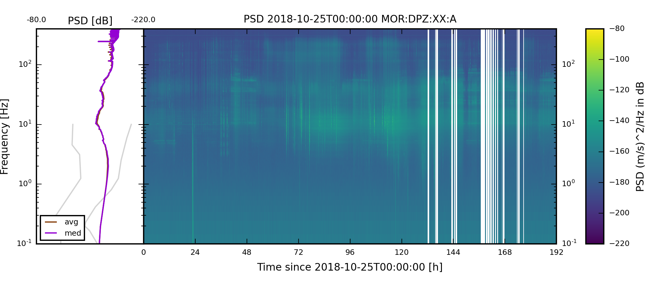
The successfully executed collection creates for each selected component a spectrogram image for the given time span and saves it in the specified output directory.

stefan@hausmeister:~/tutorial/psysmon_output/psd_images$ tree -L 4
.
└── XX
    ├── MIT
    │   └── A
    │       └── whole_20181025_20181102_XX_MIT_A_DPZ.png
    └── MOR
        └── A
            └── whole_20181025_20181102_XX_MOR_A_DPZ.png

5 directories, 2 files
stefan@hausmeister:~/tutorial/psysmon_output/psd_images$ 

The spectrogram images should look like the following images.

Create weekly spectrograms

Reopen the preferences dialog of the create psd images collection node and change the plot mode to weekly.

Execute the collection and check the weekly images created in the output directory. The weekly images should have been added.

stefan@hausmeister:~/tutorial/psysmon_output/psd_images$ tree -L 4
.
└── XX
    ├── MIT
    │   └── A
    │       ├── weekly_20181022_20181029_XX_MIT_A_DPZ.png
    │       ├── weekly_20181029_20181105_XX_MIT_A_DPZ.png
    │       └── whole_20181025_20181102_XX_MIT_A_DPZ.png
    └── MOR
        └── A
            ├── weekly_20181022_20181029_XX_MOR_A_DPZ.png
            ├── weekly_20181029_20181105_XX_MOR_A_DPZ.png
            └── whole_20181025_20181102_XX_MOR_A_DPZ.png

5 directories, 6 files
stefan@hausmeister:~/tutorial/psysmon_output/psd_images$ 

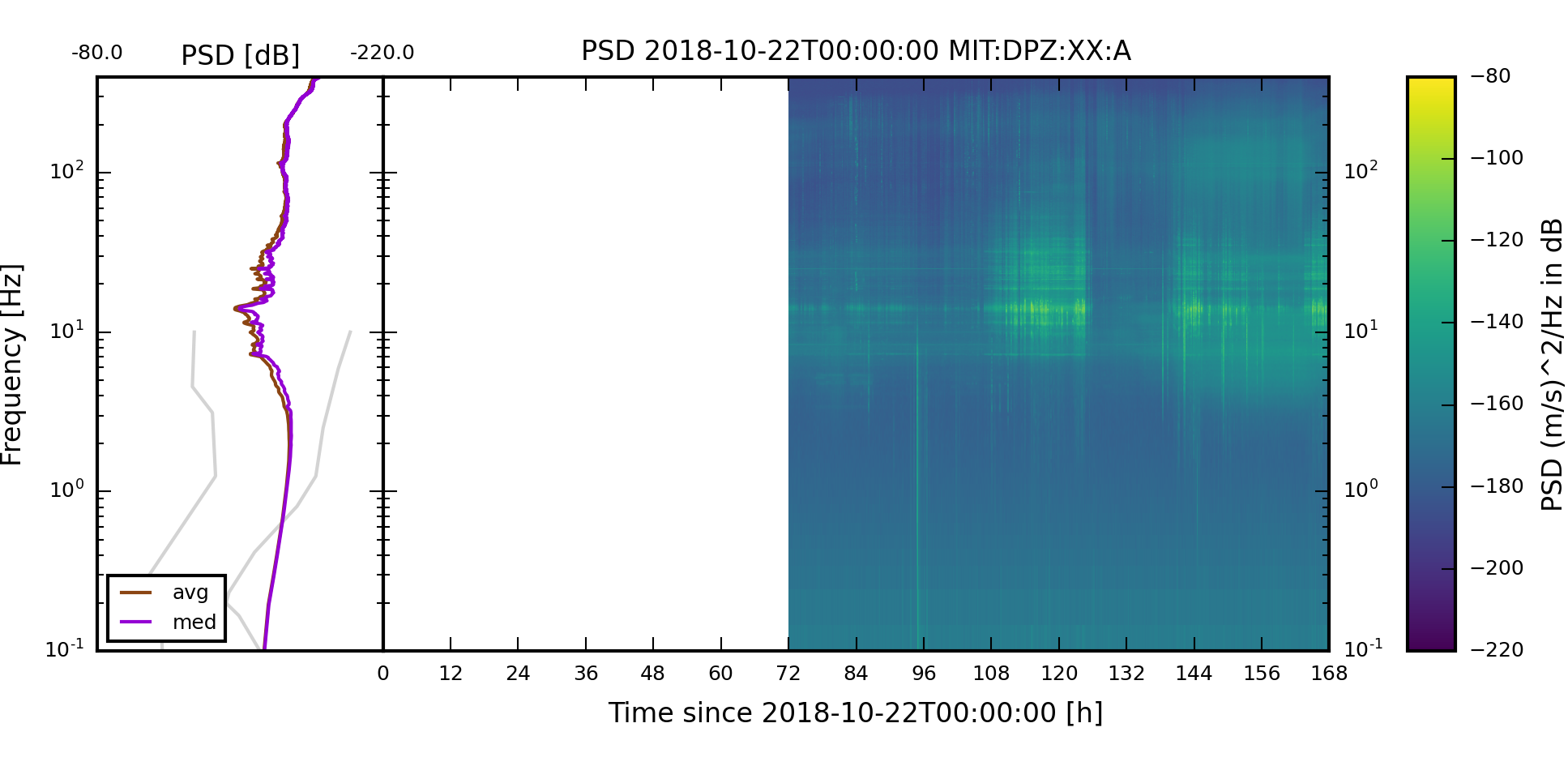
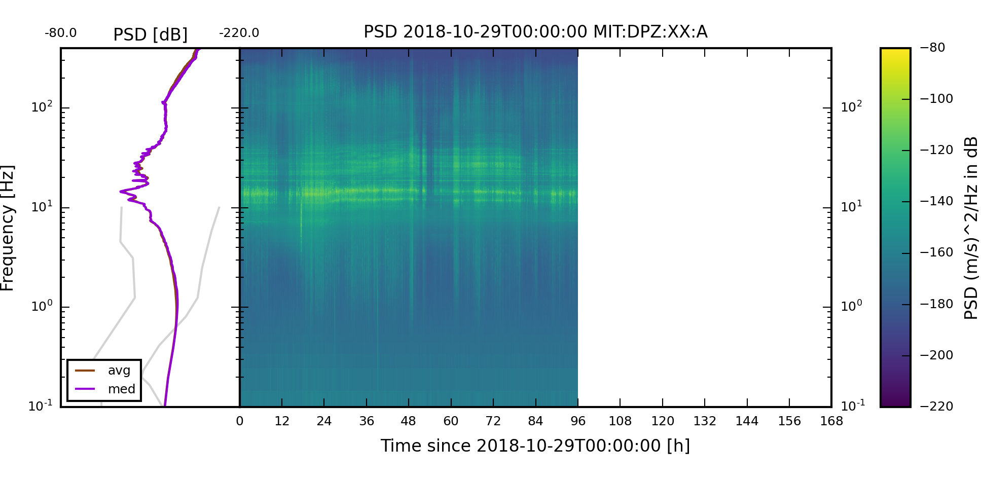
The two weekly spectrogram images of component XX:MIT:A:DPZ should look like the follwing two images. The weekly plots always start on a Monday.

Copyright © 2022 Stefan Mertl.

This article is licensed under a Creative Commons Attribution-ShareAlike 4.0 International license.

You are allowed to share the material, that means to copy and redistribute the material in any medium or format as long as you give appropriate credit to the creator and add the link to the license. You are allowed to adapt, that means to remix, transform, and build upon the material. If you adapt the material, you must distribute your contributions under the same license as the original.

If possible, please cite this article using the following form:
Psysmon Documentation, Sonnblick Events, "PSD Visualization", Stefan Mertl, 2022-08-27, www.mertl-research.at, licensed under CC BY-SA 4.0