Creating probability power spectral density plots.

Probability Power Spectral Density

The Probability Power Spectral Density (PPSD) plots are a well known method to assess the data quality of seismic data. The PPSD data computed with psysmon can be used to create PPSD plots for various time spans.

On this page

A standard procedure when analyzing the seismic data is to compute spectrograms and the probability power spectral density (PPSD) of the recorded data [1]. This gives a good overview of the general behaviour of the ambient seismic noise and reveals periods with changes in the frequency or amplitude characteristics. It also provides a good temporal compression without loosing significant information and large data sets can be screened very fast for phases of special interest.

The compute PPSD looper child node provides the computation of the PPSD images using the obspy PPSD class. In contrast to the computation of the PSD, the PPSD computation is not yet split into creating the data first and then the images. The images and the data are created by the compute PPSD looper child node in one go.

Create the output directory

Again, create an output directory to save the data of the PPSD computation. Create the directory ppsd in the psysmon_output directory of the tutorial directory structure.

stefan@hausmeister:~/tutorial/psysmon_output$ mkdir ppsd
stefan@hausmeister:~/tutorial/psysmon_output$ tree -L 1
.
├── availability
├── ppsd
├── psd_data
└── psd_images

4 directories, 0 files
stefan@hausmeister:~/tutorial/psysmon_output$ 

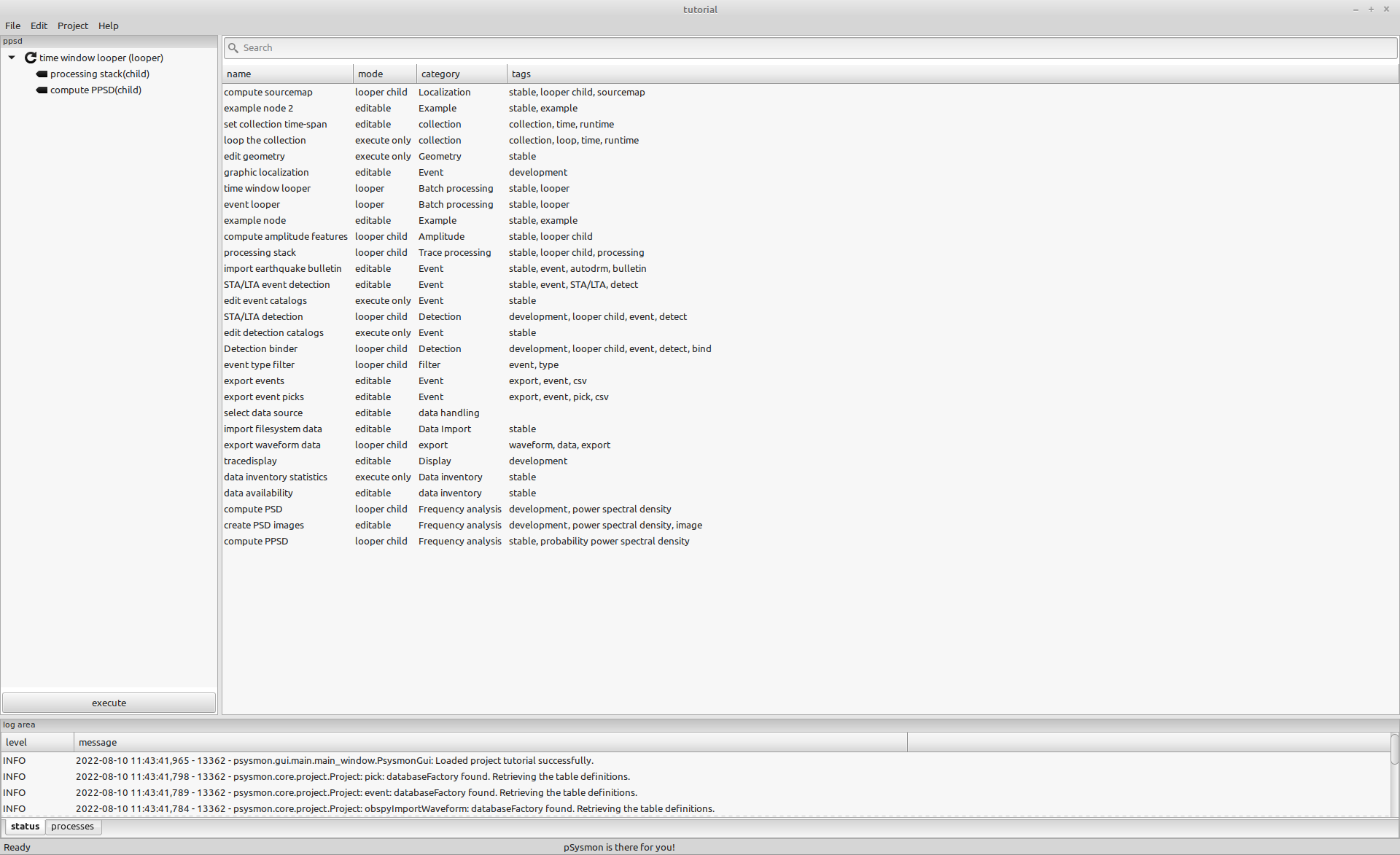
Create the ppsd collection

Create a collection named ppsd and add the collection node time window looper to the collection. Then select the time window looper node in the collection listbox and add the processing stack and then the compute PPSD looper collection node. Both of these nodes are looper children and will be added to the time window looper as child-nodes. Check the correct order of the child-nodes. The ‘processing stack’ should be on top of the ‘compute PPSD’ node.

The ppsd collection with the time window looper collection node with the processing stack and the compute ppsd looper children.

Configure the time window looper

Open the preferences editor of the time window looper using the context menu.

The time window looper splits the specified time range into time windows and executes the child-nodes for each time window.

The goal is to compute daily PPSD images for your data set.

To keep the execution fast, select only the two components MIT:XX:A:DPZ and MOR:XX:A:DPZ.

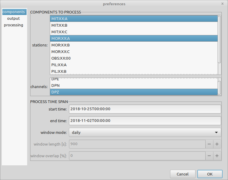
Components

Set the following preferences in the components panel:

stations: MIT:XX:AA, MOR:XX:AA
channels: DPZ
start time: 2018-10-25T00:00:00
end time: 2018-11-02T00:00:00
window mode: daily
window length: This parameter has no effect on the daily window mode. It is disabled.
window overlap: This parameter has no effect on the daily window mode. It is disabled.

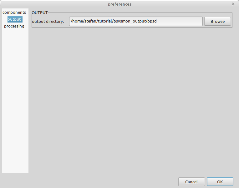
The time window looper components preferences.

Output

Set the following preferences in the output panel:

output directory: The ppsd output directory createds above.

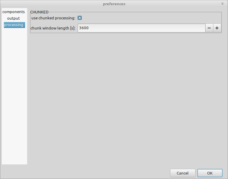
The time window looper output preferences.

Processing

For this time, chunked processing is used to create the PPSD images. Chunked processing splits up the time windows of the time window looper. The individual chunks with length chunk window lenght are subsequently fed to the child-nodes. If a looper child node support chunked processing, like compute ppsd does, the chunks are processed individually and accumulated by the child node to produce one single result per sliding window.

When loading data for long sliding windows (e.g. daily or weekly), the chunked processing option reduces the memory demand and increases execution speed. If chunked processing is not supported by the child node, each passed data chunk will be handled individually without considering an accumulation of the chunks.

In our example, the daily time windows of the time window looper will be split up into chunks with a length of 3600 seconds. Only the data of one chunk will be loaded and then fed to the looper child nodes. The processing stack applys the selected processing nodes to the individual chunk. No chunked processing is supported by the processing stack. The compute PPSD looper child node adds the chunk to the obspy PPSD computation until all chunks of a looper time window are processed. At the end, one PPSD image of the daily time window is created.

Set the following preferences in the processing panel:

use chunked processing: checked
chunk window length: 3600

The time window looper processing preferences.

Configure the processing stack child node

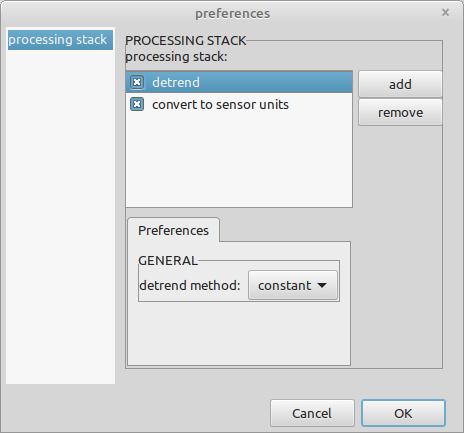
Select the processing stack node in the sub-tree of the time window looper and open the preferences editor using the context menu.

The processing stack is the same as the one that we already encountered in the tracedisplay when screening the seismic data. Add the convert to sensor units processing node to the processing stack using the add button and selecting the node from the opening dialog.

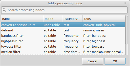
Select the convert to sensor units processing node.

The processing node will be added to the processing stack in the preferences dialog.

The convert to sensor units processing node added to the processing stack.

The convert to sensor units will convert the counts of the digital seismogram to the sensor input unit of the sensor specified in the geometry file. For the sensors used in the tutorial data set these unit is velocity (m/s). The conversion is done using the preamplification and bitweight of the data recorder and the sensitivity of the sensor. The effects of the transfer function of the sensor are not removed.

The conversion from counts to sensor units is important to relate the computed PSD data to the global noise models when creating the PPSD images.

Configure the compute ppsd child node.

Open the preferences editor of the compute ppsd child node using the context menu. The preferences dialog of the compute ppsd will open.

The computation of the PPSD removes the influence of the sensor transfer function, but it doesn’t convert the counts to the sensor units using the sensor sensitivity. This has to be done using the processing stack as described above.

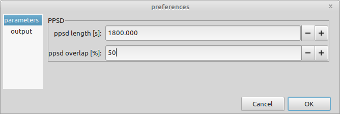
Parameters

These parameters will be passed to the obspy PPSD computation class.

Set the following preferences in the parameters panel:

ppsd length: 1800
ppsd overlap: 50

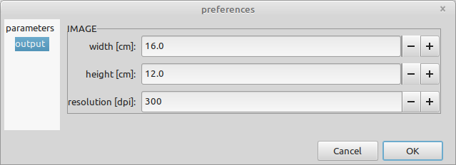
The parameters page of the compute ppsd child node preferences editor.

Output

Set the following preferences in the output panel:

width: 16
height: 12
resolution: 300

The output page of the compute ppsd child node preferences editor.

Start the computation

To start the computation of the PPSD images and data, execute the ppsd collection by clicking the execute button. A new process will be started. You can check the execution of the ppsd collection using the log file of the process.

The compute ppsd child node will create a directory structure in the specified output directory where the PPSD images and the related data is saved.

The PPSD output data

The PPSD images and data are saved as daily files in the specified output directory.

stefan@hausmeister:~/tutorial/psysmon_output/ppsd/smi-mr.sm-psysmon-tutorial-ppsd_20220810_144656_496132-time_window_looper/ppsd$ tree -L 3
.
├── images
│   ├── MIT
│   │   └── DPZ
│   └── MOR
│       └── DPZ
└── ppsd_objects
    ├── MIT
    │   └── DPZ
    └── MOR
        └── DPZ

10 directories, 0 files
stefan@hausmeister:~/tutorial/psysmon_output/ppsd/smi-mr.sm-psysmon-tutorial-ppsd_20220810_144656_496132-time_window_looper/ppsd$ cd images/MIT
stefan@hausmeister:~/tutorial/psysmon_output/ppsd/smi-mr.sm-psysmon-tutorial-ppsd_20220810_144656_496132-time_window_looper/ppsd/images/MIT$ tree -L 2
.
└── DPZ
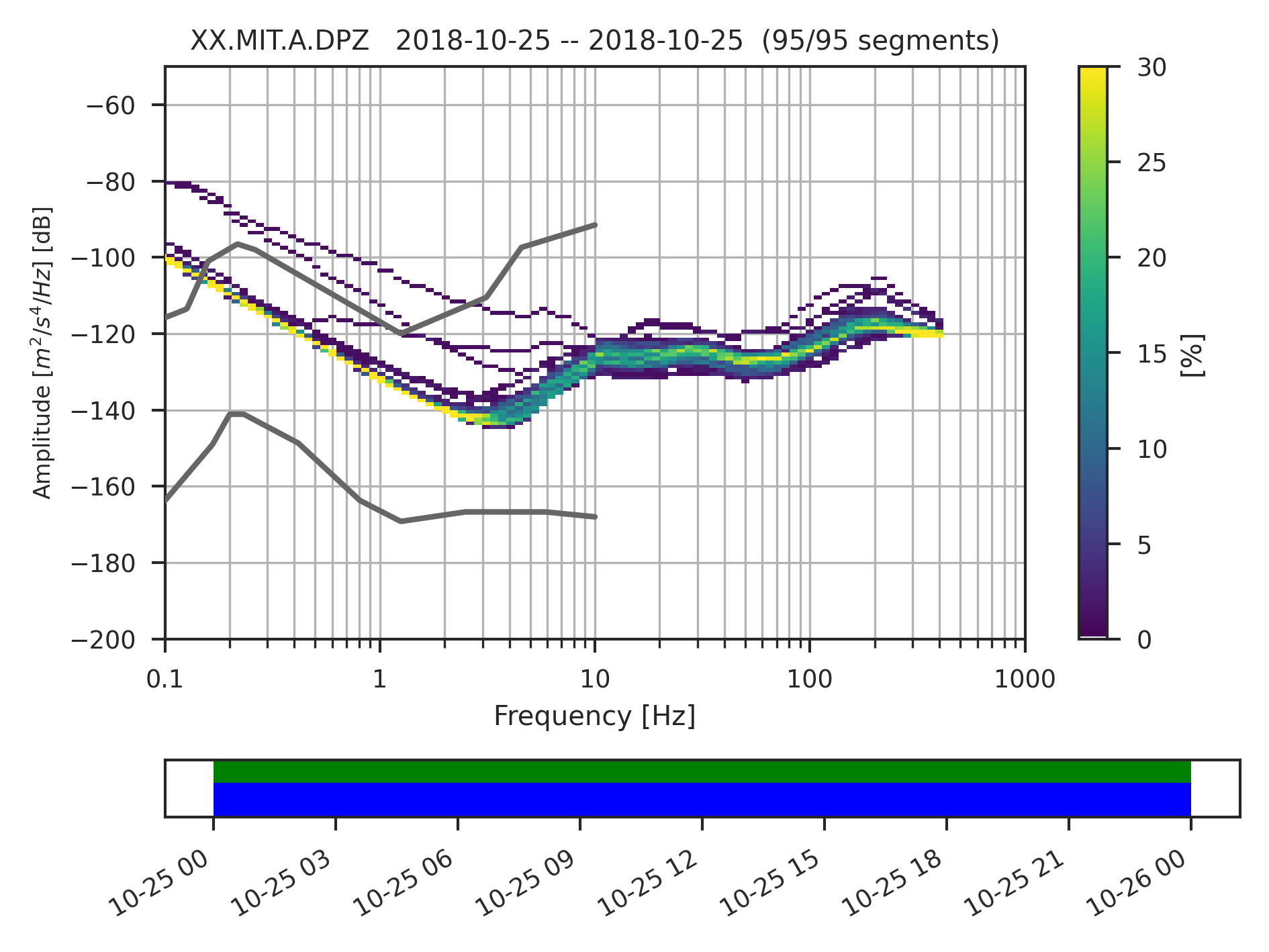
    ├── ppsd_XX_MIT_A_DPZ_2018-10-25T000000_2018-10-26T000000.png
    ├── ppsd_XX_MIT_A_DPZ_2018-10-26T000000_2018-10-27T000000.png
    ├── ppsd_XX_MIT_A_DPZ_2018-10-27T000000_2018-10-28T000000.png
    ├── ppsd_XX_MIT_A_DPZ_2018-10-28T000000_2018-10-29T000000.png
    ├── ppsd_XX_MIT_A_DPZ_2018-10-29T000000_2018-10-30T000000.png
    ├── ppsd_XX_MIT_A_DPZ_2018-10-30T000000_2018-10-31T000000.png
    ├── ppsd_XX_MIT_A_DPZ_2018-10-31T000000_2018-11-01T000000.png
    └── ppsd_XX_MIT_A_DPZ_2018-11-01T000000_2018-11-02T000000.png

1 directory, 8 files
stefan@hausmeister:~/tutorial/psysmon_output/ppsd/smi-mr.sm-psysmon-tutorial-ppsd_20220810_144656_496132-time_window_looper/ppsd/images/MIT$ cd ../../ppsd_objects/MIT
stefan@hausmeister:~/tutorial/psysmon_output/ppsd/smi-mr.sm-psysmon-tutorial-ppsd_20220810_144656_496132-time_window_looper/ppsd/ppsd_objects/MIT$ tree -L 2
.
└── DPZ
    ├── ppsd_XX_MIT_A_DPZ_2018-10-26T000000_2018-10-26T000000.pkl.npz
    ├── ppsd_XX_MIT_A_DPZ_2018-10-27T000000_2018-10-27T000000.pkl.npz
    ├── ppsd_XX_MIT_A_DPZ_2018-10-28T000000_2018-10-28T000000.pkl.npz
    ├── ppsd_XX_MIT_A_DPZ_2018-10-29T000000_2018-10-29T000000.pkl.npz
    ├── ppsd_XX_MIT_A_DPZ_2018-10-30T000000_2018-10-30T000000.pkl.npz
    ├── ppsd_XX_MIT_A_DPZ_2018-10-31T000000_2018-10-31T000000.pkl.npz
    ├── ppsd_XX_MIT_A_DPZ_2018-11-01T000000_2018-11-01T000000.pkl.npz
    └── ppsd_XX_MIT_A_DPZ_2018-11-02T000000_2018-11-02T000000.pkl.npz

1 directory, 8 files
stefan@hausmeister:~/tutorial/psysmon_output/ppsd/smi-mr.sm-psysmon-tutorial-ppsd_20220810_144656_496132-time_window_looper/ppsd/ppsd_objects/MIT$ 

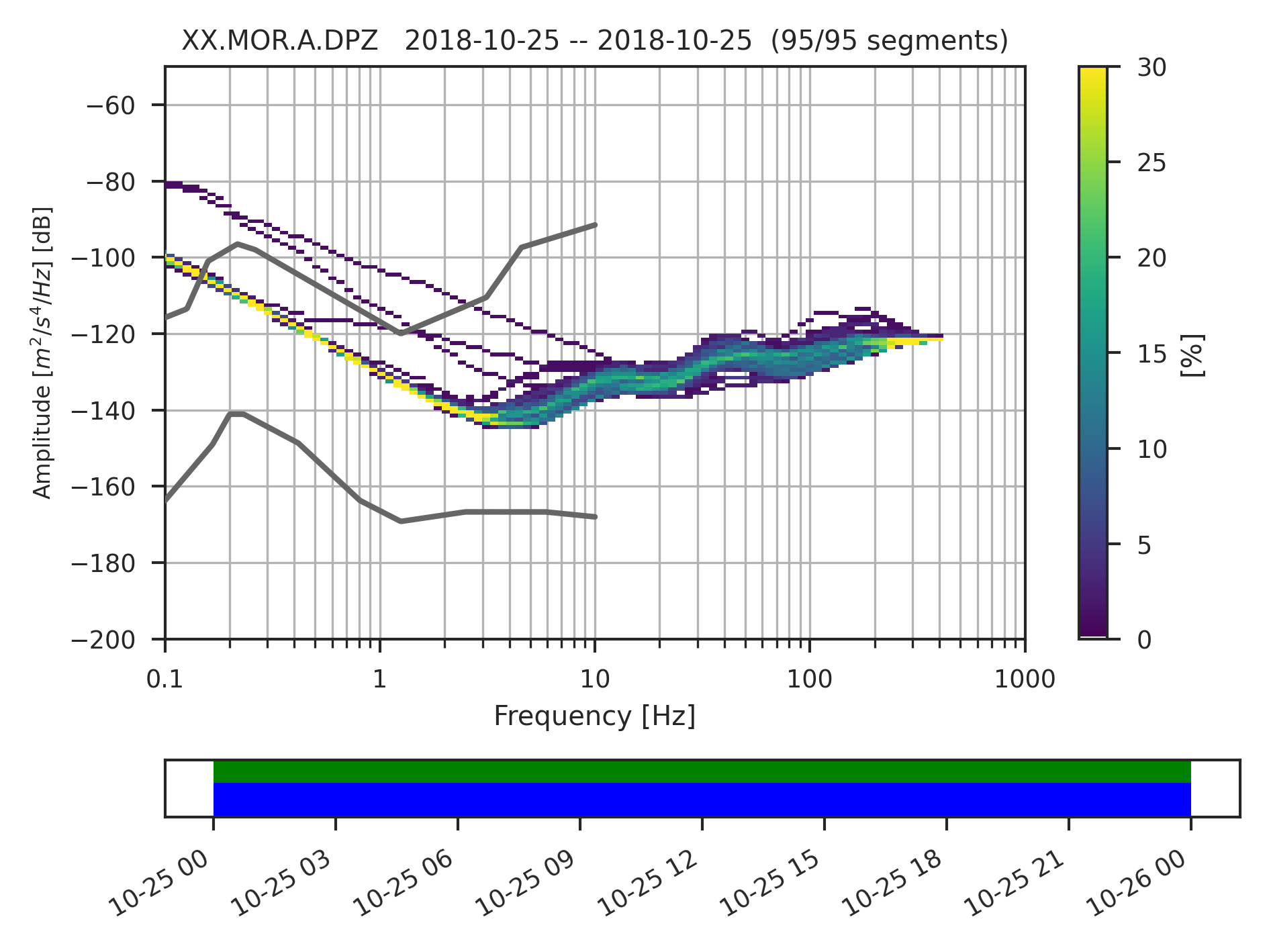
Example PPSD images

PPSD image for station MIT.

PPSD image for station MOR.

References

D. E. McNamara and R. P. Buland, “Ambient Noise Levels in the Continental United States,” Bulletin of the Seismological Society of America, vol. 94, no. 4, pp. 1517–1527, 2004.

http://doi.org/10.1785/012003001 http://www.bssaonline.org/content/94/4/1517.abstract

@article{mcnamara_ambient_2004,
  title = {Ambient Noise Levels in the Continental United States},
  volume = {94},
  url = {http://www.bssaonline.org/content/94/4/1517.abstract},
  doi = {10.1785/012003001},
  pages = {1517--1527},
  number = {4},
  journaltitle = {Bulletin of the Seismological Society of America},
  author = {McNamara, Daniel E. and Buland, Raymond P.},
  year = {2004},
  file = {mcnamara_buland_2004_ambient_noise_levels_in_the_continental_united_states.pdf:/home/stefan/01_gtd/05_dokumente/bibliothek/zotero/storage/TXUJREZB/mcnamara_buland_2004_ambient_noise_levels_in_the_continental_united_states.pdf:application/pdf}
}

This article is licensed under a Creative Commons Attribution-ShareAlike 4.0 International license.

You are allowed to share the material, that means to copy and redistribute the material in any medium or format as long as you give appropriate credit to the creator and add the link to the license. You are allowed to adapt, that means to remix, transform, and build upon the material. If you adapt the material, you must distribute your contributions under the same license as the original.

If possible, please cite this article using the following form:
Psysmon Documentation, Sonnblick Events, "Probability Power Spectral Density", Stefan Mertl, 2022-08-27, www.mertl-research.at, licensed under CC BY-SA 4.0