Computation of the power spectral density.

Power Spectral Density

Long term spectrograms are useful to evaluate the data quality and periods of special interest. psysmon provides the tools to compute the power spectral density (PSD) for the complete data set which then can be used to create spectrograms for the desired time spans.

On this page

psysmon provides so-called looper collection nodes that allow the creation of iterative execution of the looper child nodes. Currently the time window looper and the event looper are available. For the task to compute the power spectral density (PSD) for the whole data set we will use the time window looper which enables the processing of sliding time windows.

The aim of the PSD computation is to create long-term spectrogram images of the complete data set. Therefore we will first compute the PSD for 15 minute long time windows with an overlap of 50 % and then use these PSDs to create the spectrogram images for the desired time span.

Create the output directory

We will save the PSD data in a dedicated output directory for later use. Create the directory psd_data in the psysmon_output folder of the tutorial directory structure.

stefan@hausmeister:~/tutorial$ cd psysmon_output/
stefan@hausmeister:~/tutorial/psysmon_output$ mkdir psd_data
stefan@hausmeister:~/tutorial/psysmon_output$ tree -L 1
.
├── availability
└── psd_data

2 directories, 0 files
stefan@hausmeister:~/tutorial/psysmon_output$ 

Create the psd collection

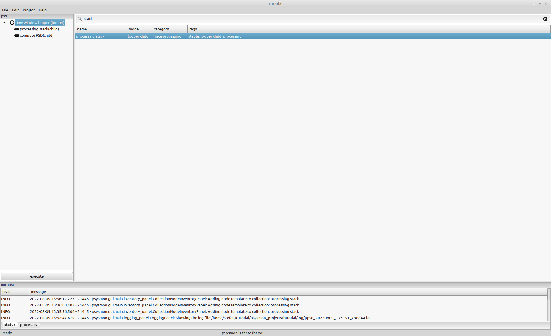
Create a collection named psd and add the collection node time window looper to the collection. Then select the time window looper node in the collection listbox and add the processing stack and then the compute PSD looper collection node. Both of these nodes are looper children and will be added to the time window looper as sub-nodes.

The time window looper splits a selected time range into time windows and for which the child nodes of the looper are executed individually.

The psd collection with the time window looper collection node with the processing stack and the compute psd looper children.

Configure the time window looper

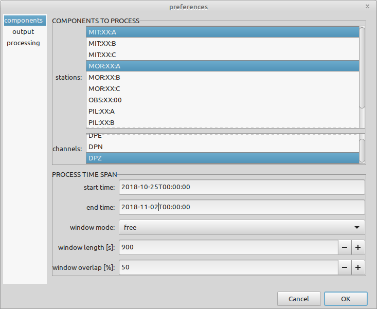
As we have defined above, we aim for sliding time windows with a length of 900 seconds and an overlap of 50 %. We will set the time window looper preferences accordingly. To keep the execution fast, we will select only the components MIT:XX:A:DPZ and MOR:XX:A:DPZ.

Set the following preferences in the components panel:

stations: MIT:XX:AA, MOR:XX:AA
channels: DPZ
start time: 2018-10-25T00:00:00
end time: 2018-11-02T00:00:00
window mode: free
window length: 900
window overlap: 50

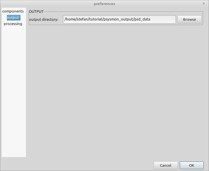
The component preferences of the time window looper collection node.

Set the following preferences in the output panel:

output directory: The tutorial/psysmon_output/psd_data directory on your file system.

The output preferences of the time window looper collection node.

Keep the default values of the processing panel.

Configure the processing stack child node

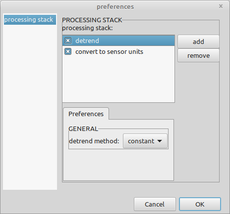
Select the processing stack node in the sub-tree of the time window looper and open the preferences editor using the context menu.

Open the preferences dialog of the time window looper child node using the context menu.

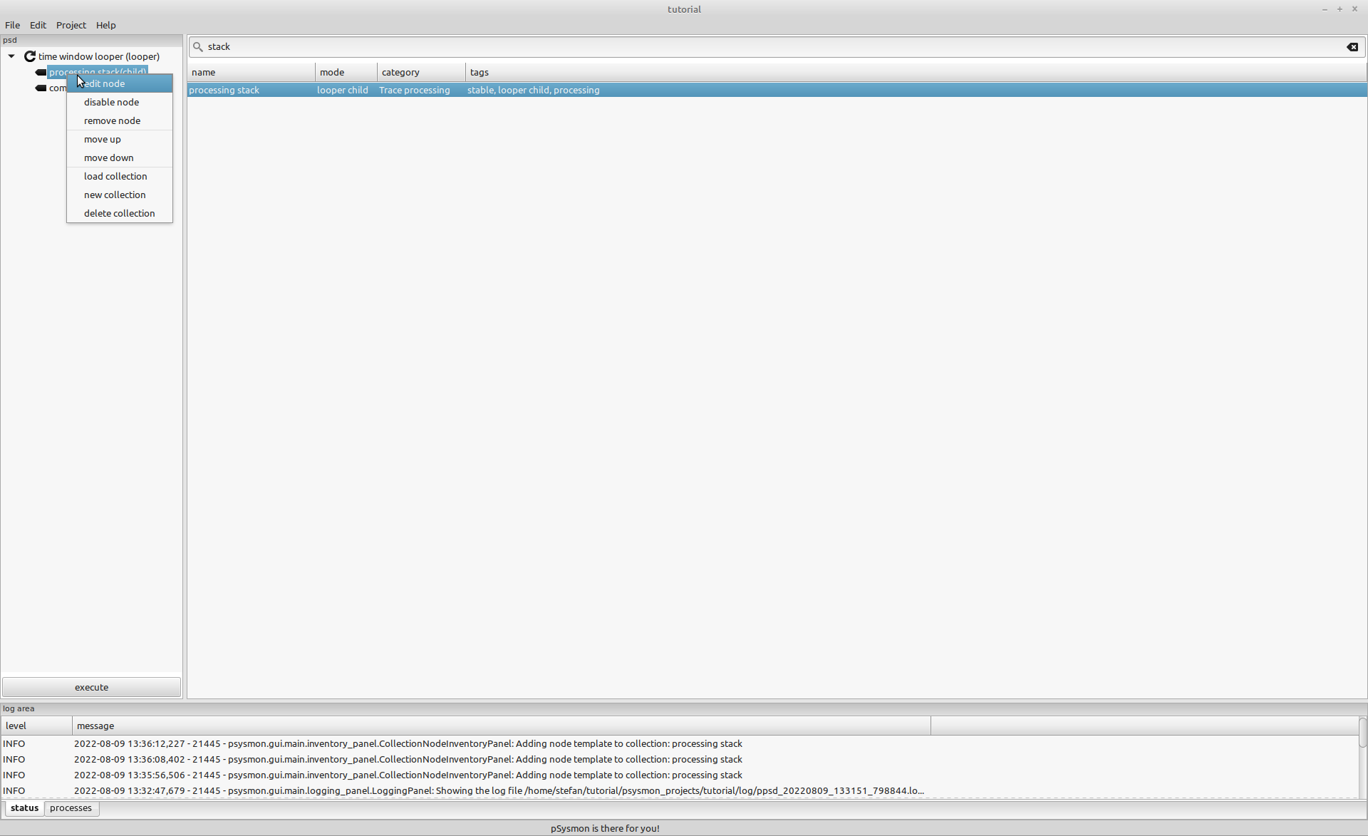
The preferences dialog of the processing stack child node opens.

The processing stack is the same as the one that we already encountered in the tracedisplay when screening the seismic data. Click the add button in the preferences dialog to open another dialog with all the available processing nodes. Select the convert to sensor units processing node and add it to the processing stack using the add button.

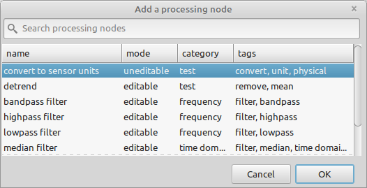
Select the convert to sensor units processing node.

The processing node is now added to the processing stack in the preferences dialog.

The convert to sensor units processing node added to the processing stack.

The convert to sensor units converts the counts of the digital seismogram to the sensor input unit specified in the geometry file. The sensor input unit for the tutorial data set is velocity (m/s). The conversion employs the preamplification and bitweight of the data recorder, and the sensitivity of the sensor. The effects of the transfer function of the sensor are not removed.

The conversion from counts to sensor units is important to relate the computed PSD data to the global noise models when creating the spectrogram images.

Configure the compute PSD child node

Select the compute PSD node in the collection node and open the preferences editor using the context menu.

The compute PSD node uses the matplotlib.mlab.psd function of matplotlib to compute the PSD data. It uses the Welch’s average periodogram method to compute the PSD for a long time series. The vector of data points passed to the psd function is divided into segments with a length of nfft samples. An overlap can be specified for the segments. You can check the source code of the compute PSD node in the psysmon github repository for more details about the computation.

We will use the default values for this node. The nfft value sets the number of spectral points used for the Fourier Transform and the fft overlap gives the overlap of these segments used in the Welch’s average periodogram method. The nfft length and the fft overlap is not related to the time window length and overlap of the time window looper. For our example the PSD will be computed for each 900 seconds long time window which the time window looper passes to the compute PSD node.

Check the values and make sure that the values are the following:

nfft: 8192
fft overlap [%]: 50

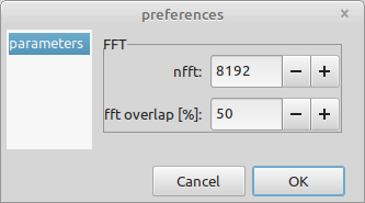
Set the preferences of the compute PSD looper child node.

Confirm the preferences by clicking the OK button.

Start the computation

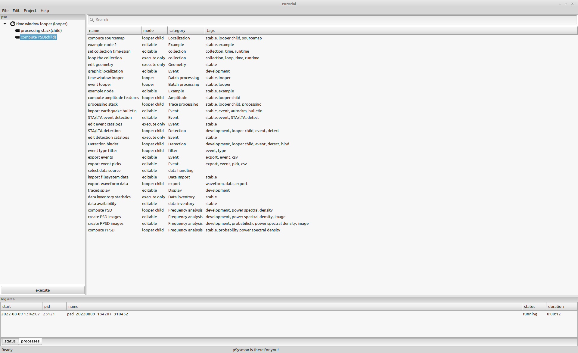
To start the computation of the PSD data, execute the collection by clicking the Execute button. A new process will be started, but no dialog window will be opened. You can check the execution of the psd collection using the log file of the process.

The collection will create a directory structure in the output directory of the time window looper where the PSD data is saved as Python shelve files.

Tracking a process using the log file

You can track a collection execution process using the Linux tail command. First, get the filename of the log file of the process that you want to check. It is built using the process name and the .log file suffix. The screenshot below shows the log file output of the running process with the name psd_20220808_152407_255098. The process log files can be found in the directory psysmon_projects/tutorial/log of your tutorial directory structure. Use the -f flag of the tail command to follow the updates of the log file.

Get the log filename from the currently running process in the log area.

stefan@hausmeister:~/tutorial/psysmon_projects/tutorial/log$ tail -f psd_20220809_134207_310452.log 
#LOG# - 2022-08-09 13:44:44,457 - INFO - psysmon.packages.core_looper.time_window_looper.SlidingWindowProcessor: Processing sliding window 1117/1536.
#LOG# - 2022-08-09 13:44:44,458 - INFO - psysmon.packages.core_looper.time_window_looper.SlidingWindowProcessor: Initial stream request for time-span: 2018-10-30T19:30:00 to 2018-10-30T19:45:00 for scnl: [('MIT', 'DPZ', 'XX', 'A'), ('MOR', 'DPZ', 'XX', 'A')].
#LOG# - 2022-08-09 13:44:44,487 - INFO - psysmon.packages.frequency.compute_psd.ComputePsdNode: ###Processing trace with id XX.MIT.A.DPZ.
#LOG# - 2022-08-09 13:44:44,505 - INFO - psysmon.packages.frequency.compute_psd.ComputePsdNode: ###Processing trace with id XX.MOR.A.DPZ.
#LOG# - 2022-08-09 13:44:44,523 - INFO - psysmon.packages.core_looper.time_window_looper.SlidingWindowProcessor: Processing sliding window 1118/1536.
#LOG# - 2022-08-09 13:44:44,523 - INFO - psysmon.packages.core_looper.time_window_looper.SlidingWindowProcessor: Initial stream request for time-span: 2018-10-30T19:37:30 to 2018-10-30T19:52:30 for scnl: [('MIT', 'DPZ', 'XX', 'A'), ('MOR', 'DPZ', 'XX', 'A')].
#LOG# - 2022-08-09 13:44:44,551 - INFO - psysmon.packages.frequency.compute_psd.ComputePsdNode: ###Processing trace with id XX.MIT.A.DPZ.
^C
stefan@hausmeister:~/tutorial/psysmon_projects/tutorial/log$ 

The PSD output data

The psd collection saves the computation results in a directory structure within the output directory specified in the time window looper node. The data is saved in hourly files organized in daily directories for each selected component. These data files are used as an input for the computation of the long-term spectrogram images.

stefan@hausmeister:~/tutorial/psysmon_output/psd_data/smi-mr.sm-psysmon-tutorial-psd_20220809_134207_310452-time_window_looper$ tree -L 2 psd
psd
├── MIT
│   └── DPZ
└── MOR
    └── DPZ

4 directories, 0 files
stefan@hausmeister:~/tutorial/psysmon_output/psd_data/smi-mr.sm-psysmon-tutorial-psd_20220809_134207_310452-time_window_looper$ tree -L 1 psd/MIT/DPZ
psd/MIT/DPZ
├── 2018_298
├── 2018_299
├── 2018_300
├── 2018_301
├── 2018_302
├── 2018_303
├── 2018_304
└── 2018_305

8 directories, 0 files
stefan@hausmeister:~/tutorial/psysmon_output/psd_data/smi-mr.sm-psysmon-tutorial-psd_20220809_134207_310452-time_window_looper$ tree -L 1 psd/MIT/DPZ/2018_298
psd/MIT/DPZ/2018_298
├── psd_20181025T000000_20181025T005230_MIT_DPZ_XX_A.db
├── psd_20181025T010000_20181025T015230_MIT_DPZ_XX_A.db
├── psd_20181025T020000_20181025T025230_MIT_DPZ_XX_A.db
├── psd_20181025T030000_20181025T035230_MIT_DPZ_XX_A.db
├── psd_20181025T040000_20181025T045230_MIT_DPZ_XX_A.db
├── psd_20181025T050000_20181025T055230_MIT_DPZ_XX_A.db
├── psd_20181025T060000_20181025T065230_MIT_DPZ_XX_A.db
├── psd_20181025T070000_20181025T075230_MIT_DPZ_XX_A.db
├── psd_20181025T080000_20181025T085230_MIT_DPZ_XX_A.db
├── psd_20181025T090000_20181025T095230_MIT_DPZ_XX_A.db
├── psd_20181025T100000_20181025T105230_MIT_DPZ_XX_A.db
├── psd_20181025T110000_20181025T115230_MIT_DPZ_XX_A.db
├── psd_20181025T120000_20181025T125230_MIT_DPZ_XX_A.db
├── psd_20181025T130000_20181025T135230_MIT_DPZ_XX_A.db
├── psd_20181025T140000_20181025T145230_MIT_DPZ_XX_A.db
├── psd_20181025T150000_20181025T155230_MIT_DPZ_XX_A.db
├── psd_20181025T160000_20181025T165230_MIT_DPZ_XX_A.db
├── psd_20181025T170000_20181025T175230_MIT_DPZ_XX_A.db
├── psd_20181025T180000_20181025T185230_MIT_DPZ_XX_A.db
├── psd_20181025T190000_20181025T195230_MIT_DPZ_XX_A.db
├── psd_20181025T200000_20181025T205230_MIT_DPZ_XX_A.db
├── psd_20181025T210000_20181025T215230_MIT_DPZ_XX_A.db
├── psd_20181025T220000_20181025T225230_MIT_DPZ_XX_A.db
└── psd_20181025T230000_20181025T235230_MIT_DPZ_XX_A.db

0 directories, 24 files
stefan@hausmeister:~/tutorial/psysmon_output/psd_data/smi-mr.sm-psysmon-tutorial-psd_20220809_134207_310452-time_window_looper$ 

This article is licensed under a Creative Commons Attribution-ShareAlike 4.0 International license.

You are allowed to share the material, that means to copy and redistribute the material in any medium or format as long as you give appropriate credit to the creator and add the link to the license. You are allowed to adapt, that means to remix, transform, and build upon the material. If you adapt the material, you must distribute your contributions under the same license as the original.

If possible, please cite this article using the following form:
Psysmon Documentation, Sonnblick Events, "Power Spectral Density", Stefan Mertl, 2022-08-27, www.mertl-research.at, licensed under CC BY-SA 4.0